Discrete simulation methods for recrystallization and grain growth

Introduction to discrete recrystallization and grain growth simulation

The design of time and space discretized recrystallization models for predicting texture and microstructure in the course of materials processing which predict kinetics and energies in a local fashion are of interest for two reasons. First, from a fundamental point of view it is desirable to understand better the dynamics and the topology of microstructures that arise from the interaction of large numbers of lattice defects which are characterized by a wide spectrum of intrinsic properties and interactions in spatially heterogeneous materials under complex engineering boundary conditions. For instance, in the field of recrystallization (and grain growth) the influence of local grain boundary characteristics (mobility, energy), local driving forces, and local crystallographic textures on the final microstructure is of particular interest. An important point of interest in that context, however, is the question how local such a models should be in its spatial discretization in order to really provide microstructural input that cannot be equivalently provided by statistical methods. In the worst case a problem in that field may be that spatially discrete recrystallization models may have the tendency to pretend a high degree of precision without actually providing it. In other words even in highly discretized recrystallization models the physics always lies in the details of the constitutive description of the kinetics and thermodynamics of the deformation structure and of the interfaces involved. The mere fact that a model is formulated in a discrete fashion does not, as a rule, automatically render it a sophisticated model per se. Second, from a practical point of view it makes sense to predict microstructure parameters such as the crystal size or the crystallographic texture which determine the mechanical and physical properties of materials subjected to industrial processes on a sound phenomenological basis.

Cellular automaton models of recrystallization

Cellular automata are algorithms that describe the discrete spatial and temporal evolution of complex systems by applying local transformation rules to lattice cells which typically represent volume portions. The state of each lattice site is characterized in terms of a set of internal state variables. For recrystallization models these can be lattice defect quantities (stored energy), crystal orientation, or precipitation density. Each site assumes one out of a finite set of possible discrete states. The opening state of the automaton is defined by mapping the initial distribution of the values of the chosen state variables onto the lattice.

The dynamical evolution of the automaton takes place through the application of deterministic or probabilistic transformation rules (switching rules) that act on the state of each lattice point. These rules determine the state of a lattice point as a function of its previous state and the state of the neighboring sites. The number, arrangement, and range of the neighbor sites used by the transformation rule for calculating a state switch determines the range of the interaction and the local shape of the areas which evolve. Cellular automata work in discrete time steps. After each time interval the values of the state variables are updated for all points in synchrony mapping the new (or unchanged) values assigned to them through the transformation rule. Owing to these features, cellular automata provide a discrete method of simulating the evolution of complex dynamical systems which contain large numbers of similar components on the basis of their local interactions.

Cellular automata are – like all other continuum models that work above the discrete atomic scale – not intrinsically calibrated by a characteristic physical length or time scale. This means that a cellular automaton simulation of continuum systems requires the definition of elementary units and transformation rules that adequately reflect the kinetics at the level addressed. If some of the transformation rules refer to different real time scales (e.g. recrystallization and recovery, bulk diffusion and grain boundary diffusion) it is essential to achieve a correct common scaling of the entire system. The requirement for an adjustment of time scaling among various rules is due to the fact that the transformation behavior of a cellular automaton is sometimes determined by non-coupled Boolean routines rather than by local solutions of coupled differential equations.

The following examples on the use of cellular automata for predicting recrystallization textures are designed as automata with a probabilistic transformation rule. Independent variables are time and space. The latter is discretized into equally shaped cells each of which is characterized in terms of the mechanical driving force (stored deformation energy) and the crystal orientation (texture). The starting data of such automata are usually derived from experiment (for instance from a microtexture map) or from plasticity theory (for instance from crystal plasticity finite element simulations). The initial state is typically defined in terms of the distribution of the crystal orientation and of the driving force. Grains or subgrains are mapped as regions of identical crystal orientation, but the driving force may vary inside these areas.

The kinetics of the automaton gradually evolve from changes in the state of the cells (cell switches). They occur in accord with a switching rule (transformation rule) which determines the individual switching probability of each cell as a function of its previous state and the state of its neighbor cells. The switching rule is designed to map the phenomenology of primary static recrystallization. It reflects that the state of a non-recrystallized cell belonging to a deformed grain may change due to the expansion of a recrystallizing neighbor grain which grows according to the local driving force and boundary mobility. If such an expanding grain sweeps a non-recrystallized cell the stored dislocation energy of that cell drops to zero and a new orientation is assigned to it, namely that of the expanding neighbor grain. The mathematical formulation of the automaton used in this report can be found in. It is derived from a probabilistic form of a linearized symmetric rate equation, which describes grain boundary motion in terms of isotropic single-atom diffusion processes perpendicular through a homogeneous planar grain boundary segment under the influence of a decrease in Gibbs energy. This means that the local progress in recrystallization can be formulated as a function of the local driving forces (stored deformation energy) and interface properties (grain boundary mobility). The most intricate point in such simulations consists in identifying an appropriate phenomenological rule for nucleation events.

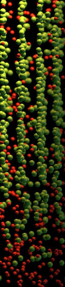
The movie above shows an example of a coupling of a cellular automaton with a crystal plasticity finite element model for predicting recrystallization textures in Aluminium. The major advantage of such an approach is that it considers the inherited material deformation heterogeneity as opposed to material homogeneity.

This type of coupling the two models, therefore, seems more appropriate when aiming at the simulation of textures formed during materials processing. Nucleation in this coupled simulation works above the subgrain scale, i.e. it does not explicitly describe cell walls and subgrain coarsening phenomena. Instead, it incorporates nucleation on a more phenomenological basis using the kinetic and thermodynamic instability criteria known from classical recrystallization theory. The kinetic instability criterion means that a successful nucleation process leads to the formation of a mobile high angle grain boundary which can sweep the surrounding deformed matrix. The thermodynamic instability criterion means that the stored energy changes across the newly formed high angle grain boundary providing a net driving force pushing it forward into the deformed matter. Nucleation in this simulation is performed in accord with these two aspects, i.e. potential nucleation sites must fulfill both, the kinetic and the thermodynamic instability criterion. The used nucleation model does not create any new orientations. At the beginning of the simulation the thermodynamic criterion, i.e. the local value of the dislocation density was first checked for all lattice points. If the dislocation density was larger than some critical value of its maximum value in the sample, the cell was spontaneously recrystallized without any orientation change, i.e. a dislocation density of zero was assigned to it and the original crystal orientation was preserved. In the next step the conventional cellular growth algorithm was used, i.e. the kinetic conditions for nucleation were checked by calculating the misorientations among all spontaneously recrystallized cells (preserving their original crystal orientation) and their immediate neighborhood considering the first, second, and third neighbor shell. If any such pair of cells revealed a misorientation above 15°, the cell flip of the unrecrystallized cell was calculated according to its actual transformation probability. In case of a successful cell flip the orientation of the first recrystallized neighbor cell was assigned to the flipped cell.

See also further contents here:

The cellular automaton simulation method

Examples of recrystallization models

Potts-type Monte Carlo multi-spin models of recrystallization

The application of the Metropolis Monte Carlo method in microstructure simulation has gained momentum particularly through the extension of the Ising lattice model for modeling magnetic spin systems to the kinetic multistate Potts lattice model. The original Ising model is in the form of an ½ spin lattice model where the internal energy of a magnetic system is calculated as the sum of pair-interaction energies between the continuum units which are attached to the nodes of a regular lattice. The Potts model deviates from the Ising model by generalizing the spin and by using a different Hamiltonian. It replaces the Boolean spin variable where only two states are admissible (spin up, spin down) by a generalized variable which can assume one out of a larger spectrum ofdiscrete possible ground states, and accounts only for the interaction between dissimilar neighbors. The introduction of such a spectrum of different possible spins enables one to represent domains discretely by regions of identical state (spin). For instance, in microstructure simulation such domains can be interpreted as areas of similarly oriented crystalline matter. Each of these spin orientation variables can be equipped with a set of characteristic state variable values quantifying the lattice energy, the dislocation density, the Taylor factor, or any other orientation-dependent constitutive quantity of interest. Lattice regions which consist of domains with identical spin or state are in such models translated as crystal grains. The values of the state variable enter the Hamiltonian of the Potts model. The most characteristic property of the energy operator when used for coarsening models is that it defines the interaction energy between nodes with like spins to be zero, and between nodes with unlike spins to be one. This rule makes it possible to identify interfaces and to quantify their energy as a function of the abutting domains.

The kinetic evolution of the Potts model which occurs in the form of domain growth is usually simulated using Metropolis or Glauber dynamics, i.e. it proceeds by randomly selecting lattice sites, switching their orientational state randomly to a new one, and weighting the resulting energy change in terms of Metropolis Monte Carlo sampling. This means that an orientation flip is generally accepted if it leads to a state of lower or equal energy and is accepted with thermal probability if it leads to an energy increase.

The Potts model is very versatile for describing coarsening phenomena. It takes a quasi-microscopic metallurgical view of grain growth or ripening, where the crystal interior is composed of lattice points (e.g. atom clusters) with identical energy (e.g. orientation) and the grain boundaries are the interfaces between different types of such domains. As in a real ripening scenario, interface curvature leads to increased wall energy on the convex side and thus to wall migration entailing local shrinkage. The discrete simulation steps in the Potts model, by which the system proceeds towards thermodynamic equilibrium, are typically calculated by randomly switching lattice sites and weighting the resulting interfacial energy changes in terms of Metropolis Monte Carlo sampling.

Vertex models of recrystallization

Vertex and related front tracking simulations are another alternative for engineering process models with respect to recrystallization phenomena. Their use is currently less common when compared to the widespread application of Monte Carlo and cellular automaton models owing to their geometrical complexity and the required small integration time steps. Despite these differences to lattice based recrystallization models they have an enormous potential for predicting interface dynamics at small scales also in the context of process simulations.

Topological network and vertex models idealize solid materials or soap-like structures as homogeneous continua which contain interconnected boundary segments that meet at vertices, i.e. boundary junctions. Depending on whether the system dynamics lies in the motion of the junctions or of the boundary segments, they are sometimes also referred to as boundary dynamics or, more generalized, as front tracking models. The grain boundaries appear as lines or line segments in two-dimensional and as planes or planar segments in three-dimensional simulations. The dynamics of these coupled interfaces or interface portions and of the vertices determine the evolution of the entire network.

The dynamical equations of the boundary and node (vertex) motion can be described in terms of a damped Newtonian equation of motion which contains a large frictional portion or, mathematically equivalent, in terms of a linearized first-order rate equation. Using the frictional form of the classical equation of motion with a strong damping term results in a steady-state motion where the velocity of the defect depends only on the local force but not on its previous velocity. The over-damped steady-state description is similar to choosing a linearized rate equation, where the defect velocity is described in terms of a temperature-dependent mobility term and the local driving pressure.

The calculation of the local forces in most vertex models is based on equilibrating the line energies of subgrain walls and high-angle grain boundaries at the interface junctions according to Herring’s equation. The enforcement of the local mechanical equilibrium at these nodes is for obvious topological reasons usually only possible by allowing the abutting interfaces to curve.

These curvatures in turn act through their capillary force, which is directed towards the center of curvature, on the junctions. In sum this may lead to their displacement. In order to avoid the artificial enforcement of a constant boundary curvature between two neighboring nodes, the interfaces are usually decomposed into sequences of piecewise straight boundary segments.

Most vertex and network models use switching rules which describe the topological recombination of approaching vertices when such neighboring nodes are closer than some critical spontaneous recombination spacing. This is an analogy to the use of phenomenological annihilation and lock-formation rules that appear in dislocation dynamics. As in all continuum models, the use of such empirical recombination laws replaces a more exact atomistic treatment.

It is worth noting in this context that the recombination rules, particularly the various values for the critical recombination spacing of specific configurations, can affect the topological results of a simulation. Depending on the underlying constitutive continuum description, vertex simulations can consider crystal orientation and, hence, misorientations across the boundaries, interface mobility, and the difference in elastic energy between adjacent grains. Due to the stereological complexity of grain boundary arrays and the large number of degrees of freedom encountered in such approaches, most network simulations are currently confined to the two-dimensional regime. Topological boundary dynamics models are different from kinetic cellular automaton or Potts Monte Carlo models in that they are not based on minimizing the total energy but directly calculate the motion of the lattice defects, usually on the basis of capillary and elastic forces.